Machine learning models can be pretty impressive — sometimes almost magical — when you see them in action. They can diagnose diseases, control robots, or even help scientists design new materials, as shown in some recent examples. But they’re not perfect. Every now and then, a model behaves in strange ways. That’s why it’s worth asking not only what a model predicts, but how confident it is about those predictions.
This is where probabilistic machine learning comes in. Instead of giving just one answer, these models tell us a range of possible answers along with how likely each one is. One of the most powerful and elegant tools for this is the Gaussian Process (GPs).
What is a Gaussian process?
Mathematically, according to Wikipedia, a Gaussian process is a stochastic process where any collection of points has a joint multivariate normal distribution. A fuller and much more practical explanation can be found in Rasmussen and Williams’ excellent book.
In simple terms, a GP says: for every input \(x\), instead of a single, fixed output \(f(\mathbf{x})\), we have a distribution described by a mean function \(\mu(x)\) and a covariance function \(\text{cov}(x, x')\). The mean tells us the “average” prediction, and the covariance tells us how predictions for different inputs are related.
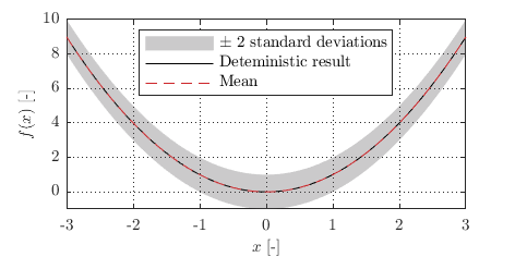
 For example, if \(f(x) = x^2\) is a deterministic function, a stochastic version might keep the same mean \(\mu(x) = x^2\) but add uncertainty with \(\text{cov}(x, x') = 0.5^2 I\), where \(I\) is the identity matrix.
How to make it useful
The main idea in machine learning is to design a model, feed it with data, and tweak it so that its predictions match reality as closely as possible. As George Box famously put it: “All models are wrong, but some are useful.”
With Gaussian Processes, the process starts with defining a prior — a set of assumptions about what the function might look like before seeing any data.
Step 1: Create the model
A GP is defined by a mean function and a covariance function (also called a kernel). In many cases, we set the mean to zero, \(\mu(x) = 0\), without losing generality, and focus on choosing the right kernel.
One of the most popular and versatile kernels is the Squared Exponential (SE) kernel:
\[k(x, x') = \sigma_s^2 \exp\left( -\frac{1}{2} \frac{(x - x')^2}{\ell^2} \right),\]with \(\sigma_s\) controlling the vertical scale (how much the function values can vary overall), and \(\ell\) being the lengthscale, which says how far you need to move in \(x\) before you expect a big change in \(y\).
If the data have noise, we can add a noise term:
\[k(x, x') = \sigma_s^2 \exp\left( -\frac{1}{2} \frac{(x - x')^2}{\ell^2} \right) + \sigma_n^2 \delta(x, x'),\]where \(\sigma_n\) is the noise level and \(\delta\) is the Kronecker delta. This basically adds a little uncertainty to the diagonal of the covariance matrix, making the predictions less rigid around the observed points.
In this case, the kernel type and the parameters \(\sigma_s\), \(\ell\), and \(\sigma_n\) completely define your prior.
Step 2: Bring in the data
Once we have a prior, the next step is to update it with observed data. This is where Bayes’ theorem comes in. It tells us how to combine what we believed before seeing the data (the prior) with what the data suggest (the likelihood) to get an updated belief (the posterior):
\[p(f(\mathbf{x}) \mid \mathcal{D}) = \frac{p(\mathcal{D} \mid f(\mathbf{x})) \, p(f(\mathbf{x}))}{p(\mathcal{D})}.\]Here:
- \(f (\mathbf{x})\) is the unknown function we’re modelling.
- \(\mathcal{D} = \{ \mathbf{x}, \mathbf{y} \}\) is the training data (inputs and outputs).
- \(p(f(\mathbf{x}))\) is the prior — what we believe about \(f\) before seeing any data.
- \(p(\mathcal{D} \mid f(\mathbf{x}))\) is the likelihood — how probable it is to see our data if the true function were \(f (\mathbf{x})\).
- \(p(f(\mathbf{x}) \mid \mathcal{D})\) is the posterior — the updated distribution over functions after seeing the data.
- \(p(\mathcal{D})\) is the evidence or marginal likelihood — it normalises the posterior so probabilities sum to 1.
For Gaussian Process regression, we usually assume the observations are noisy but Gaussian-distributed around the true function values. This means the likelihood is:
\[p(\mathbf{y} \mid f, \mathbf{x}) = \mathcal{N}\left( \mathbf{y} \,\middle|\, f(\mathbf{x}), \sigma_n^2 I \right).\]When you combine a Gaussian prior with a Gaussian likelihood, something interesting happens: the posterior is also Gaussian, and the math works out in closed form. That’s one of the reasons GPs are so appealing — we get exact Bayesian inference without resorting to approximations.
Learning in GPs relates to the process of finding the optimal values of the free model parameters (in this case, \(\sigma_s\), \(\ell\), and \(\sigma_n\)). This is usually done by maximisation of the Gaussian likelihood shown above.
The result is a posterior distribution over functions that agrees with our prior where we have no data, and hugs the data points closely where we do have measurements, with uncertainty shrinking near observations and growing in between them.
Step 3: See it in action
The interactive example below shows how a GP works in practice. You can change the kernel parameters and see how the prior changes. Then, by clicking on the plot, you can add data points and watch how the model adapts.
