One of the best things about probabilistic machine learning is that it doesn’t just give you an answer — it tells you how sure it is about that answer. Gaussian processes (GPs) are the go-to model for this because they treat unknown functions as probability distributions, and they let us do some really handy things like conditioning on data, taking derivatives, and keeping all the maths neat and analytical.

Now, if you take a GP and combine it with the actual equations that describe your physical system, you get what’s called a physics-informed Gaussian process. In this post, you’ll see how we can combined the Euler–Bernoulli beam equation with a multi-output GP to jointly work out deflections, rotations, strains, and internal forces in a beam — and even update uncertain material parameters — straight from observed data. This has been presented during the IABSE Symposium in Prague, CZ. A preprint of the paper is available at arXiv.

Modelling the Euler–Bernoulli beam with a multi-output GP

The Euler–Bernoulli equation relates a beam’s bending stiffness \(EI\) to its deflection \(u(x)\) and applied load \(q(x)\) via a fourth-order differential equation:

\[EI\,\frac{\mathrm{d}^4 u(x)}{\mathrm{d} x^4} = q(x),\]

where \(x \in [0,L]\) represents the longitudinal coordinate of a beam of length \(L\).

A zero-mean GP prior is placed on the deflection: \(u(x) \sim \mathcal{GP}(0, k_{uu}(x,x')),\) with a squared exponential kernel \(k_{uu}(x,x') = \sigma_s^2 \exp\left(-\tfrac{1}{2}\frac{(x - x')^2}{\ell^2}\right),\) where \(\sigma_s\) is the vertical scale and \(\ell\) is the characteristic lengthscale.

Because the beam equation is linear, derivatives of the GP are still GPs. Differentiating the kernel four times yields the covariance function for the load \(q(x)\), while fewer derivatives produce covariances for rotation, curvature, bending moment, and shear force.

All outputs are collected into: \(f(x) = [u, \theta, \kappa, M, V, q]^{\mathsf{T}},\) with:

• \(\theta = \mathrm{d}u/\mathrm{d}x\) (rotation),
• \(\kappa = \mathrm{d}^2u/\mathrm{d}x^2\) (curvature),
• \(M = EI\,\kappa\) (bending moment),
• \(V = \mathrm{d}M/\mathrm{d}x\) (shear force).

This formulation produces a multi-output GP with a block-structured covariance matrix derived from repeated differentiation of the base kernel. For instance, the load kernel is obtained as

\[k_{qq}(x,x') = \frac{1}{(EI)^2}\,\frac{\partial^4}{\partial x^4}\,\frac{\partial^4}{\partial x'^4}\,k_{uu}(x,x'),\]

and similar cross‑covariance functions between deflection, rotation, curvature, bending moment and shear force. Collecting these outputs into a vector \(f(x) = [u(x), \theta(x), \kappa(x), M(x), V(x), q(x)]^{\mathsf{T}}\), where \(\theta = \mathrm{d}u/\mathrm{d}x\) is the rotation, \(\kappa = \mathrm{d}^2u/\mathrm{d}x^2\) is the curvature, \(M = EI\,\kappa\) is the bending moment and \(V = \mathrm{d}M/\mathrm{d}x\) is the shear, leads to a multi‑output Gaussian process with zero mean and block‑structured covariance matrix

\[K_{pp} = \begin{pmatrix} K_{uu} & K_{u\theta} & \cdots & K_{uq} \\ K_{\theta u} & K_{\theta\theta} & \cdots & K_{\theta q} \\ \vdots & \vdots & \ddots & \cdots \\ K_{qu} & K_{q \theta} & \cdots & K_{qq}\\ \end{pmatrix},\]

where each block is obtained by differentiating the base kernel appropriate numbers of times. Measurement noise is represented by adding diagonal blocks \(\Sigma_a^2 I\) to the covariance matrix, where \(\Sigma_a\) is the standard deviation of the noise, and boundary conditions at supports are enforced by including synthetic, noise‑free observations.

Setting the parameter priors

The model uses three sets of hyperparameters:

1. Kernel parameters \(\{\sigma_s, \ell\}\)
2. Bending stiffness \(EI\)
3. Measurement noise \(\sigma_a\)

We give each of them independent priors — broad log-uniform for the kernel parameters, and uniform for \(EI\) between 10 % and 200 % of nominal. The posterior comes from combining the likelihood and priors, and I sample from it using a Metropolis–Hastings algorithm. Predictions are then averaged over these samples, so they naturally reflect parameter uncertainty.

Numerical example: cantilever beam under uniform load

The first test case involves a cantilever beam under a uniform load \(q\). The analytical deflection is \(u(x) = q\,\frac{x^2}{24\,EI}\left(x^2 - 4Lx + 6L^2\right),\) which we use as a benchmark.

Benchmark cantilever beam used for validation of the GP model.

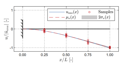
We place four virtual deflection sensors along the beam and add Gaussian noise based on a chosen signal-to-noise ratio. Then I run the MH algorithm to get posteriors for the kernel parameters, noise, and stiffness. The predicted mean deflection matches the analytical curve really well, with uncertainty growing toward the free end where the constraints imposed to the model are weaker.

Predicted deflection for the cantilever beam. Shaded area = 95 % credible interval.

Predicting of unobserved quantities

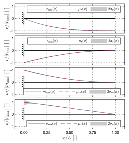
Once trained, the GP gives me not just deflection, but also rotation, curvature (or strain), bending moment, and shear force — complete with credible intervals. These line up closely with the analytical solutions, with only small increases in uncertainty near boundaries.

Predicted latent quantities — all obtained from the same GP model, even though it only trained using displacements.

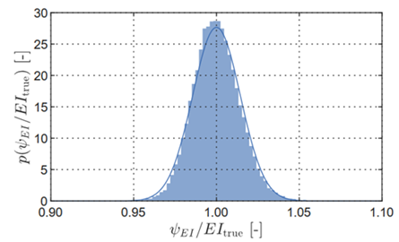
The bending stiffness estimate is also spot on, with less than 1 % bias and about 2 % relative uncertainty.

Learned structural stiffness \(\psi_{EI}\) in comparison to the true numerical stiffness \(EI_{\mathrm{true}}\)

Damage detection with Mahalanobis distance

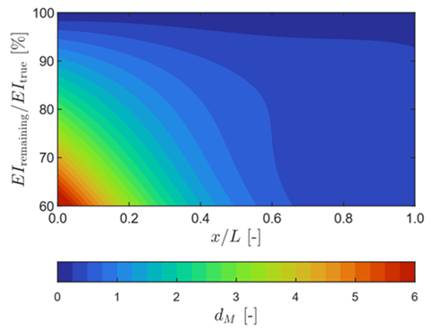
Here’s a neat trick: we simulate “damage” by reducing stiffness in one small section of the beam, then compare predicted vs. measured responses using the Mahalanobis distance \(d_M\). Large distances mean something’s off. With damage near the clamped end, the model flags it clearly; closer to the free end, it’s harder because uncertainty is higher and the effects of damage on the structural response are less pronounced.

Damage detection — larger Mahalanobis distances identify damage location and severity.

Takeaways

This physics-informed multi-output GP approach blends structural mechanics with Bayesian learning in a really natural way. By encoding the beam equation directly into the covariance, we get physically consistent predictions from sparse, noisy data, plus uncertainties on both states and parameters. It’s robust, can detect damage, and even spots dodgy sensors.

The main drawback? Computational cost grows fast with the number of data points — so high-quality, well-placed sensors are key. But it should be interesting to see extensions of this method this to plates, dynamic problems, and non-stationary kernels in the future.